Introduction
AMRgen is a comprehensive R package designed to
integrate antimicrobial resistance genotype and phenotype data. It
provides tools to:
Import AMR genotype data (e.g. from AMRFinderPlus, hAMRonization)
Import AST phenotype data (e.g. public data from NCBI or EBI, or your own data in formats like Vitek or WHOnet)
Conduct genotype-phenotype analyses to explore the impact of genotypic markers on phenotype, including via logistic regression, solo marker analysis, and upset plots
Fetch MIC or disk zone reference distributions from EUCAST
This vignette walks through a basic workflow using example datasets
included in the AMRgen package, and explains how to wrangle
your own data files into the right formats to use the same workflow.
Start by loading the package:
library(AMRgen)
library(dplyr)
#>
#> Attaching package: 'dplyr'
#> The following objects are masked from 'package:stats':
#>
#>     filter, lag
#> The following objects are masked from 'package:base':
#>
#>     intersect, setdiff, setequal, union
1. Genotype table
The import_amrfp() function lets you load genotype data
from AMRFinderPlus output files, and process it to generate an object
with the key columns needed to work with the AMRgen
package.
# Example AMRFinderPlus genotyping output (from Allthebacteria project)
ecoli_geno_raw
#> # A tibble: 45,228 × 28
#>    Name      `Protein identifier` `Contig id`  Start   Stop Strand `Gene symbol`
#>    <chr>     <lgl>                <chr>        <dbl>  <dbl> <chr>  <chr>
#>  1 SAMN0317… NA                   SAMN031776…  74721  75851 -      blaEC
#>  2 SAMN0317… NA                   SAMN031776… 166214 169315 +      acrF
#>  3 SAMN0317… NA                   SAMN031776…  20678  22033 -      glpT_E448K
#>  4 SAMN0317… NA                   SAMN031776…    758   1969 -      floR
#>  5 SAMN0317… NA                   SAMN031776…   4440   5666 +      mdtM
#>  6 SAMN0317… NA                   SAMN031776…   3941   4798 +      blaTEM-1
#>  7 SAMN0317… NA                   SAMN031776…    142    954 +      sul2
#>  8 SAMN0317… NA                   SAMN031776…   1018   1818 +      aph(3'')-Ib
#>  9 SAMN0317… NA                   SAMN031776…   1821   2654 +      aph(6)-Id
#> 10 SAMN0317… NA                   SAMN031776…    788   1957 +      tet(A)
#> # ℹ 45,218 more rows
#> # ℹ 21 more variables: `Sequence name` <chr>, Scope <chr>,
#> #   `Element type` <chr>, `Element subtype` <chr>, Class <chr>, Subclass <chr>,
#> #   Method <chr>, `Target length` <dbl>, `Reference sequence length` <dbl>,
#> #   `% Coverage of reference sequence` <dbl>,
#> #   `% Identity to reference sequence` <dbl>, `Alignment length` <dbl>,
#> #   `Accession of closest sequence` <chr>, `Name of closest sequence` <chr>, …

# Load AMRFinderPlus output
#    (replace 'ecoli_geno_raw' with the filepath for any AMRFinderPlus output)
ecoli_geno <- import_amrfp(ecoli_geno_raw, "Name")

# Check the format of the processed genotype table
head(ecoli_geno)
#> # A tibble: 6 × 36
#>   Name         gene  mutation  node  marker   marker.label drug_agent drug_class
#>   <chr>        <chr> <chr>     <chr> <chr>    <chr>        <ab>       <chr>
#> 1 SAMN03177615 blaEC NA        blaEC blaEC    blaEC        NA         Beta-lact…
#> 2 SAMN03177615 acrF  NA        acrF  acrF     acrF         NA         Efflux
#> 3 SAMN03177615 glpT  Glu448Lys glpT  glpT_E4… glpT:Glu448… FOS        Other ant…
#> 4 SAMN03177615 floR  NA        floR  floR     floR         CHL        Amphenico…
#> 5 SAMN03177615 floR  NA        floR  floR     floR         FLR        Other ant…
#> 6 SAMN03177615 mdtM  NA        mdtM  mdtM     mdtM         NA         Efflux
#> # ℹ 28 more variables: `Protein identifier` <lgl>, `Contig id` <chr>,
#> #   Start <dbl>, Stop <dbl>, Strand <chr>, `Gene symbol` <chr>,
#> #   `Sequence name` <chr>, Scope <chr>, `Element type` <chr>,
#> #   `Element subtype` <chr>, Class <chr>, Subclass <chr>, Method <chr>,
#> #   `Target length` <dbl>, `Reference sequence length` <dbl>,
#> #   `% Coverage of reference sequence` <dbl>,
#> #   `% Identity to reference sequence` <dbl>, `Alignment length` <dbl>, …
The genotype table has one row for each genetic marker detected in an input genome, i.e. one per strain/marker combination.
If your genotype data is not in AMRFinderPlus format, you can wrangle other input data files into the necessary format.
The essential columns for a genotype table to work with
AMRgen functions are:
Name: character string giving the sample name, used to link to sample names in the phenotype file (this column can have a different name, in which case you’ll need to make sure it is the first column in the dataframe OR pass its name to the functions usinggeno_sample_col)marker: character string giving the name of the genetic marker detecteddrug_class: character string giving the antibiotic class associated with this marker
NOTE: You should consider whether you have genomes with no AMR
markers detected by genotyping, and how to make sure these are include
in your analyses. E.g. AMRFinderPlus will output one row per
genome/marker combination, but if you have a genome with no markers
detected, there will be no row at all for that genome in the
concatenated output file. If your species has core genes included in
AMRFinderPlus this probably won’t be a problem as you would expect some
calls for every genome (e.g. AMRFinderPlus will report blaSHV, oqxA,
oqxB, fosA in all Klebsiella pneumoniae genomes, so all input genomes
will appear in the concatenated output file). An easy solution is to run
a check to make sure that all genome names in your input dataset are
represented in the genotype table, and if any are missing add empty rows
for these using
e.g. tibble(Name=missing_samples) %>% bind_rows(genotype_table).
2. Phenotype table
The import_ncbi_ast() function imports AST data from
NCBI format files.
# Example E. coli AST data from NCBI
# This one has already been imported and phenotypes interpreted from assay data
# You can make your own from different file formats, and interpret against breakpoints, using:
#    import_ast("filepath/NCBI_AST.tsv", format="ncbi", interpret_clsi=T)
#    import_ast("filepath/Vitek_AST.tsv", format="vitek", interpret_eucast=T)

ecoli_ast
#> # A tibble: 4,170 × 10
#>    id           drug_agent     mic  disk pheno_clsi ecoff guideline method
#>    <chr>        <ab>         <mic> <dsk> <sir>      <sir> <chr>     <chr>
#>  1 SAMN36015110 CIP        <128.00    NA   R          R   CLSI      NA
#>  2 SAMN11638310 CIP         256.00    NA   R          R   CLSI      NA
#>  3 SAMN05729964 CIP          64.00    NA   R          R   CLSI      Etest
#>  4 SAMN10620111 CIP         >=4.00    NA   R          R   CLSI      NA
#>  5 SAMN10620168 CIP         >=4.00    NA   R          R   CLSI      NA
#>  6 SAMN10620104 CIP         <=0.25    NA   S          R   CLSI      NA
#>  7 SAMN10620102 CIP         >=4.00    NA   R          R   CLSI      NA
#>  8 SAMN10620129 CIP         >=4.00    NA   R          R   CLSI      NA
#>  9 SAMN10620121 CIP         >=4.00    NA   R          R   CLSI      NA
#> 10 SAMN10620086 CIP         >=4.00    NA   R          R   CLSI      NA
#> # ℹ 4,160 more rows
#> # ℹ 2 more variables: pheno_provided <sir>, spp_pheno <mo>

head(ecoli_ast)
#> # A tibble: 6 × 10
#>   id           drug_agent     mic  disk pheno_clsi ecoff guideline method
#>   <chr>        <ab>         <mic> <dsk> <sir>      <sir> <chr>     <chr>
#> 1 SAMN36015110 CIP        <128.00    NA   R          R   CLSI      NA
#> 2 SAMN11638310 CIP         256.00    NA   R          R   CLSI      NA
#> 3 SAMN05729964 CIP          64.00    NA   R          R   CLSI      Etest
#> 4 SAMN10620111 CIP         >=4.00    NA   R          R   CLSI      NA
#> 5 SAMN10620168 CIP         >=4.00    NA   R          R   CLSI      NA
#> 6 SAMN10620104 CIP         <=0.25    NA   S          R   CLSI      NA
#> # ℹ 2 more variables: pheno_provided <sir>, spp_pheno <mo>
Data can be imported from various standard formats using the
import_ast function, and re-interpreted using latest
breakpoints and/or ECOFF. Use ?import_ast to see the
available formats and other options.
If your assay data is not in a standard format, you can wrangle other
input data files into the necessary format, manually and/or with the
help of the format_ast function.
?import_ast

?format_ast
The phenotype table is long form, with one row for each assay measurement, i.e. one per strain/drug combination.
The essential columns for a phenotype table to work with
AMRgen functions are:
id: character string giving the sample name, used to link to sample names in the genotype file (this column can have a different name, in which case you’ll need to make sure it is the first column in the dataframe OR pass its name to the functions usingpheno_sample_col)spp_pheno: species in the form of an AMR packagemoclass (can be created from a column with species name as string, usingAMR::as.mo(species_string))drug_agent: antibiotic name in the form of an AMR packageabclass (can be created from a column with antibiotic name as string, usingAMR::as.ab(antibiotic_string))a phenotype column, e.g. the import functions output fields
pheno_eucast,pheno_clsi,pheno_provided,ecoff: S/I/R phenotype calls in the form of an AMR packagesirclass (can be created from a column with phenotype values as string, usingAMR::as(sir_string), or generated by interpreting MIC or disk assay data usingAMR::as.sir)
If you want to do analyses with raw assay data (e.g. upset plots) you will need that data in one or both of:
mic: MIC in the form of an AMR packagemicclass (can be created from a column with assay values as string, usingAMR::as.mic(mic_string))disk: disk diffusion zone diameter in the form of an AMR packagediskclass (can be created from a column with assay values as string, usingAMR::as.disk(disk_string))
The import functions also standardise names for the following common fields:
method: The laboratory testing method (e.g., “MIC”, “disk diffusion”, “Etest”, “agar dilution”)platform: The laboratory testing platform/instrument if relevant (e.g., “Vitek”, “Phoenix”, “Sensititre”).guideline: The testing standard recorded in the input file as being used to make the provided phenotype interpretations (e.g. “CLSI”, “EUCAST”)source: An identifier for the dataset from which each data point was sourced (e.g. study or hospital name, pubmed ID, bioproject accession).
3. Plot phenotype data distribution
It is always a good idea to check the distribution of raw AST data
that we have to work with. The function assay_by_var() can
be used to plot the distribution of MIC or disk measurements, coloured
by a variable.
# Example E. coli AST data from NCBI

# Plot MIC distribution, coloured by CLSI S/I/R call
assay_by_var(pheno_table = ecoli_ast, antibiotic = "Ciprofloxacin", measure = "mic", colour_by = "pheno_clsi")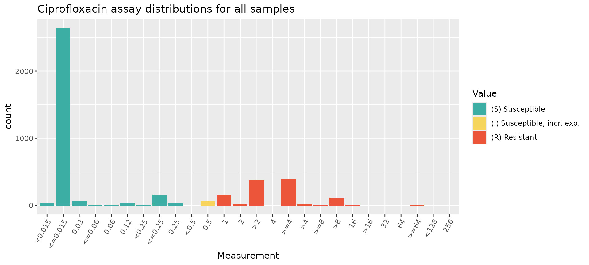
It’s a good idea to make sure that the SIR field in the
input data file has been interpreted correctly against the breakpoints.
The AMRgen function checkBreakpoints() can be used to help
look up breakpoints in the AMR package. Or, if you provide
the function assay_by_var() with a species and guideline,
it can look up the breakpoints and ECOFF and annotate these directly on
the plot.
# Look up breakpoints recorded in the AMR package
checkBreakpoints(species = "E. coli", guide = "CLSI 2025", antibiotic = "Ciprofloxacin", assay = "MIC")
#>   MIC breakpoints determined using AMR package: S <= 0.25 and R > 1
#> $breakpoint_S
#> [1] 0.25
#>
#> $breakpoint_R
#> [1] 1
#>
#> $bp_standard
#> [1] "-"

# Specify species and guideline, to annotate with CLSI breakpoints
assay_by_var(pheno_table = ecoli_ast, antibiotic = "Ciprofloxacin", measure = "mic", colour_by = "pheno_clsi", species = "E. coli", guideline = "CLSI 2025")
#>   MIC breakpoints determined using AMR package: S <= 0.25 and R > 1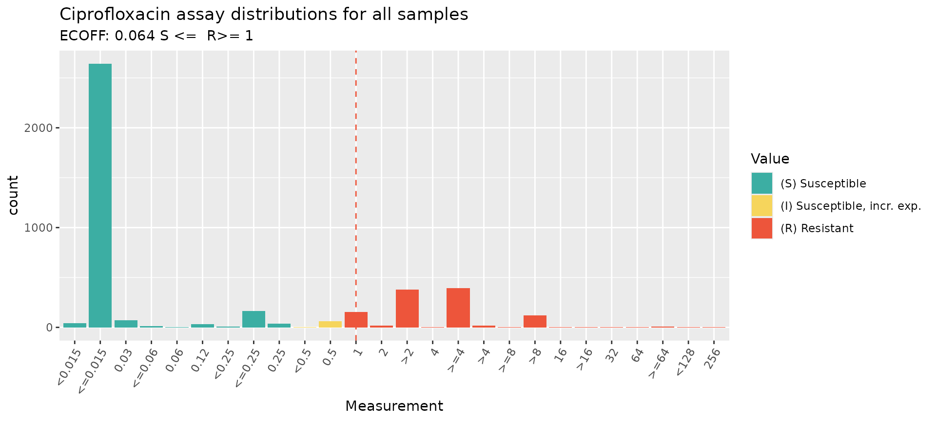
When aggregating AST data from different methods and sources, it is a
good idea to check the distributions broken down by method or source.
This can be done easily by passing the assay_by_var()
function a variable name to facet by, which means a separate
distribution will be plotted for each value of that variable (e.g. each
type of ‘method’ in our AST test data). Note that this public data from
NCBI includes non-standard values in the platform (Sensititre /
Sensititer) in the platform
# specify facet_var="method" to generate facet plots by assay method
mic_by_platform <- assay_by_var(pheno_table = ecoli_ast, antibiotic = "Ciprofloxacin", measure = "mic", colour_by = "pheno_clsi", species = "E. coli", guideline = "CLSI 2025", facet_var = "method")
#>   MIC breakpoints determined using AMR package: S <= 0.25 and R > 1

mic_by_platform$plot
#> NULL
4. Download reference assay distributions and compare to your data
It can also be helpful to check how your MIC or disk zone distribution compares to the reference distributions, to get a sense of whether your assays were calibrated correctly or if there may be some issues with a given dataset. AMRgen has functions to download the latest reference distributions from EUCAST (mic.eucast.org), and plot them on their own or with your data overlaid.
# get MIC distribution for ciprofloxacin, for all organisms
get_eucast_mic_distribution("cipro")
#> # A tibble: 2,033 × 4
#> microorganism microorganism_code mic count
#> <chr> <mo> <mic> <int>
#> 1 Achromobacter xylosoxidans B_ACHRMB_XYLS 0.002 0
#> 2 Achromobacter xylosoxidans B_ACHRMB_XYLS 0.004 0
#> 3 Achromobacter xylosoxidans B_ACHRMB_XYLS 0.008 0
#> 4 Achromobacter xylosoxidans B_ACHRMB_XYLS 0.016 0
#> 5 Achromobacter xylosoxidans B_ACHRMB_XYLS 0.030 0
#> 6 Achromobacter xylosoxidans B_ACHRMB_XYLS 0.060 0
#> 7 Achromobacter xylosoxidans B_ACHRMB_XYLS 0.125 0
#> 8 Achromobacter xylosoxidans B_ACHRMB_XYLS 0.250 1
#> 9 Achromobacter xylosoxidans B_ACHRMB_XYLS 0.500 0
#> 10 Achromobacter xylosoxidans B_ACHRMB_XYLS 1.000 6
#> # ℹ 2,023 more rows
# specify microorganism to only get results for that pathogen
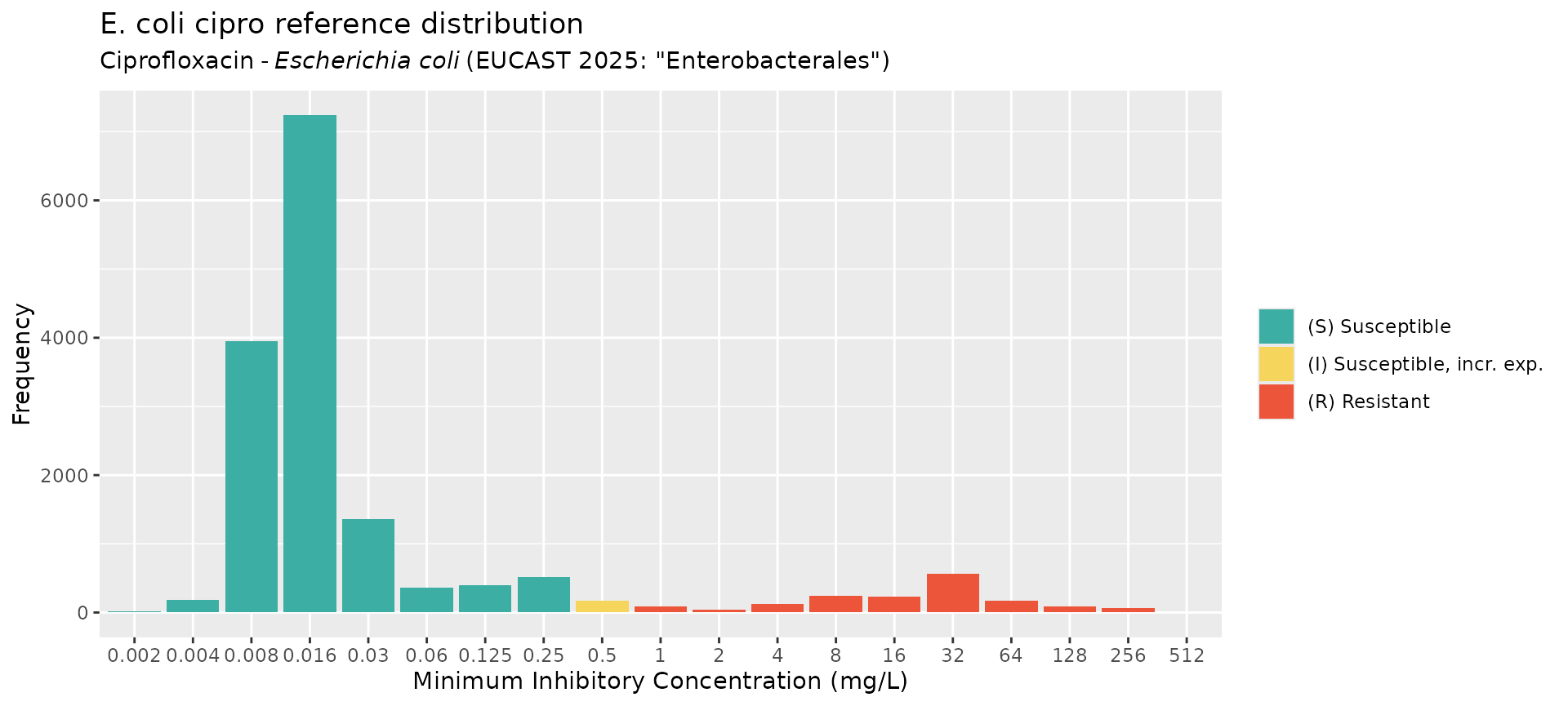
ecoli_cip_mic_data <- get_eucast_mic_distribution("cipro", "E. coli")
# get disk diffusion data instead
ecoli_cip_disk_data <- get_eucast_disk_distribution("cipro", "E. coli")
# plot the MIC data
mics <- rep(ecoli_cip_mic_data$mic, ecoli_cip_mic_data$count)
ggplot2::autoplot(
mics,
ab = "cipro",
mo = "E. coli",
title = "E. coli cipro reference distribution"
)
# Compare reference distribution to random test data
my_mic_values <- AMR::random_mic(500)
comparison <- compare_mic_with_eucast(my_mic_values, ab = "cipro", mo = "E. coli")
#> Joining with `by = join_by(value)`
comparison
#> # A tibble: 25 × 3
#>    value     user eucast
#>  * <fct>    <int>  <int>
#>  1 <=0.0005    47      0
#>  2 0.001       29      0
#>  3 0.002       44     14
#>  4 0.004       33    189
#>  5 0.008       28   3952
#>  6 0.016       34   7238
#>  7 0.03         0   1355
#>  8 0.032       24      0
#>  9 0.06         0    356
#> 10 0.064       32      0
#> # ℹ 15 more rows
#> Use ggplot2::autoplot() on this output to visualise.
ggplot2::autoplot(comparison)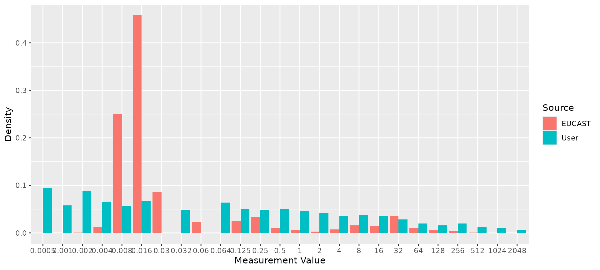
# Compare reference distribution to example E. coli data
ecoli_cip <- ecoli_ast$mic[ecoli_ast$drug_agent == "CIP"]
comparison <- compare_mic_with_eucast(ecoli_cip, ab = "cipro", mo = "E. coli")
#> Joining with `by = join_by(value)`
comparison
#> # A tibble: 34 × 3
#>    value    user eucast
#>  * <fct>   <int>  <int>
#>  1 0.002       0     14
#>  2 0.004       0    189
#>  3 0.008       0   3952
#>  4 <0.015     41      0
#>  5 <=0.015  2642      0
#>  6 0.016       0   7238
#>  7 0.03       69   1355
#>  8 <=0.06     11      0
#>  9 0.06        5    356
#> 10 0.12       34      0
#> # ℹ 24 more rows
#> Use ggplot2::autoplot() on this output to visualise.
ggplot2::autoplot(comparison)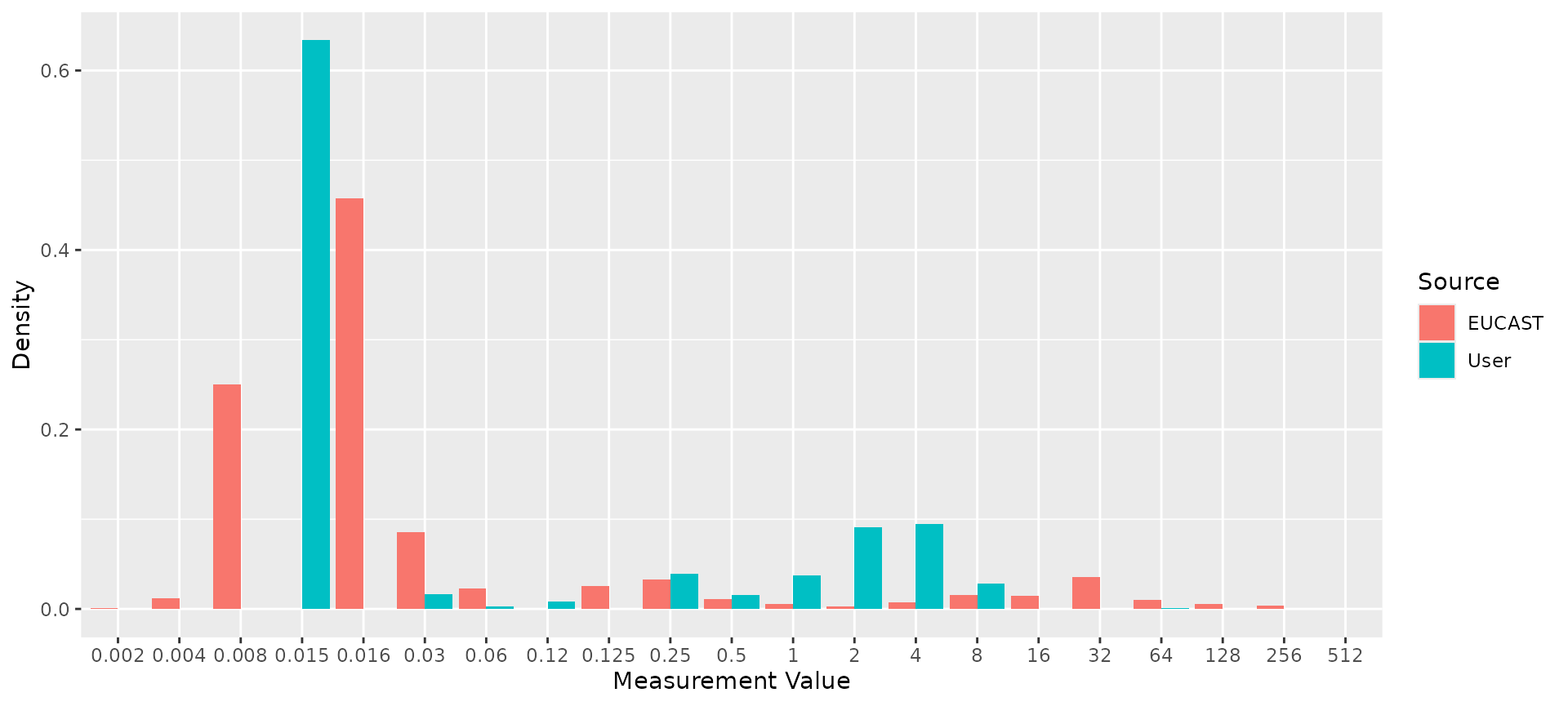
5. Combine genotype and phenotype data for a given drug
The genotype and phenotype tables can include data related to many
different drugs, but we need to analyse things one drug at a time. The
function get_binary_matrix() can be used to extract
phenotype data for a specified drug, and genotype data for markers
associated with a specified drug class. It returns a single dataframe
with one row per strain, for the subset of strains that appear in both
the genotype and phenotype input tables. Each row indicates, for one
strain, both the phenotypes (with SIR column, any assay columns if
desired, and boolean 1/0 coding of R and NWT status) and the genotypes
(one column per marker, with boolean 1/0 coding of marker
presence/absence).
# Get matrix combining phenotype data for ciprofloxacin, binary calls for R/NWT phenotype,
#    and genotype presence/absence data for all markers associated with the relevant drug
#    class (which are labelled "Quinolones" in AMRFinderPlus).
cip_bin <- get_binary_matrix(
  ecoli_geno,
  ecoli_ast,
  antibiotic = "Ciprofloxacin",
  drug_class_list = "Quinolones",
  sir_col = "pheno_clsi",
  keep_assay_values = TRUE,
  keep_assay_values_from = "mic"
)
#>  Defining NWT in binary matrix using ecoff column provided: ecoff

# check format
head(cip_bin)
#> # A tibble: 6 × 50
#>   id     pheno ecoff     mic     R   NWT gyrA_S83L gyrA_D87Y gyrA_D87N parC_S80I
#>   <chr>  <sir> <sir>   <mic> <dbl> <dbl>     <dbl>     <dbl>     <dbl>     <dbl>
#> 1 SAMN0…   S     S   <=0.015     0     0         0         0         0         0
#> 2 SAMN0…   S     S   <=0.015     0     0         0         0         0         0
#> 3 SAMN0…   S     S   <=0.015     0     0         0         0         0         0
#> 4 SAMN0…   S     R     0.250     0     1         1         0         0         0
#> 5 SAMN0…   S     R     0.120     0     1         0         1         0         0
#> 6 SAMN0…   S     S   <=0.015     0     0         0         0         0         0
#> # ℹ 40 more variables: parE_S458A <dbl>, parC_S80R <dbl>, parE_L416F <dbl>,
#> #   qnrB6 <dbl>, gyrA_D87G <dbl>, parC_S57T <dbl>, parC_E84A <dbl>,
#> #   soxS_A12S <dbl>, qnrB2 <dbl>, qnrS2 <dbl>, parC_E84K <dbl>,
#> #   parC_A56T <dbl>, qnrB19 <dbl>, `aac(6')-Ib-cr5` <dbl>, parC_E84V <dbl>,
#> #   parE_I529L <dbl>, parE_S458T <dbl>, parE_E460D <dbl>, parC_E84G <dbl>,
#> #   qnrS1 <dbl>, marR_S3N <dbl>, `aac(6')-Ib-cr` <dbl>, soxR_R20H <dbl>,
#> #   qnrB1 <dbl>, parE_I355T <dbl>, soxR_G121D <dbl>, qnrB4 <dbl>, qepA <dbl>, …

# list colnames, to see full list of quinolone markers included
colnames(cip_bin)
#>  [1] "id"             "pheno"          "ecoff"          "mic"
#>  [5] "R"              "NWT"            "gyrA_S83L"      "gyrA_D87Y"
#>  [9] "gyrA_D87N"      "parC_S80I"      "parE_S458A"     "parC_S80R"
#> [13] "parE_L416F"     "qnrB6"          "gyrA_D87G"      "parC_S57T"
#> [17] "parC_E84A"      "soxS_A12S"      "qnrB2"          "qnrS2"
#> [21] "parC_E84K"      "parC_A56T"      "qnrB19"         "aac(6')-Ib-cr5"
#> [25] "parC_E84V"      "parE_I529L"     "parE_S458T"     "parE_E460D"
#> [29] "parC_E84G"      "qnrS1"          "marR_S3N"       "aac(6')-Ib-cr"
#> [33] "soxR_R20H"      "qnrB1"          "parE_I355T"     "soxR_G121D"
#> [37] "qnrB4"          "qepA"           "gyrA_S83A"      "qnrA1"
#> [41] "parE_D475E"     "parC_A108V"     "qepA1"          "parE_E460K"
#> [45] "gyrA_S83W"      "marR_R77C"      "parE_L445H"     "parE_I464F"
#> [49] "qnrB"           "acrR_R45C"
This binary matrix can be used as the starting a lot of downstream analyses.
For example, we can use it as input to assay_by_var to
plot the assay distribution coloured by presence of a particular genetic
marker
assay_by_var(cip_bin, measure = "mic", colour_by = "parC_S80I", antibiotic = "Ciprofloxacin")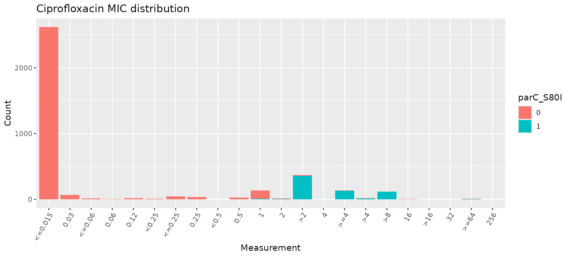
# count the number of gyrA mutations per genome
gyrA_mut <- cip_bin %>%
  dplyr::mutate(gyrA_mut = rowSums(across(contains("gyrA_") & where(is.numeric)), na.rm = T)) %>%
  select(mic, gyrA_mut)

# plot the MIC distribution, coloured by count of gyrA mutations
mic_by_gyrA_count <- assay_by_var(gyrA_mut, measure = "mic", colour_by = "gyrA_mut", colour_legend_label = "No. gyrA mutations", antibiotic = "Ciprofloxacin")

mic_by_gyrA_count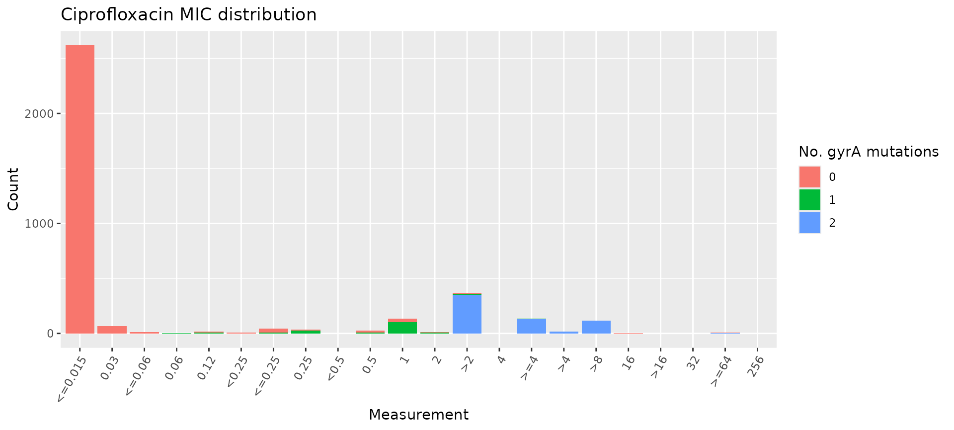
# count the number of genetic determinants per genome
marker_count <- cip_bin %>%
  mutate(marker_count = rowSums(across(where(is.numeric) & !any_of(c("R", "NWT"))), na.rm = T)) %>%
  select(mic, marker_count)

# plot the MIC distribution, coloured by count of associated genetic markers
mic_by_marker_count <- assay_by_var(marker_count, measure = "mic", colour_by = "marker_count", colour_legend_label = "No. markers detected", antibiotic = "Ciprofloxacin", bar_cols = viridisLite::viridis(max(marker_count$marker_count) + 1))

mic_by_marker_count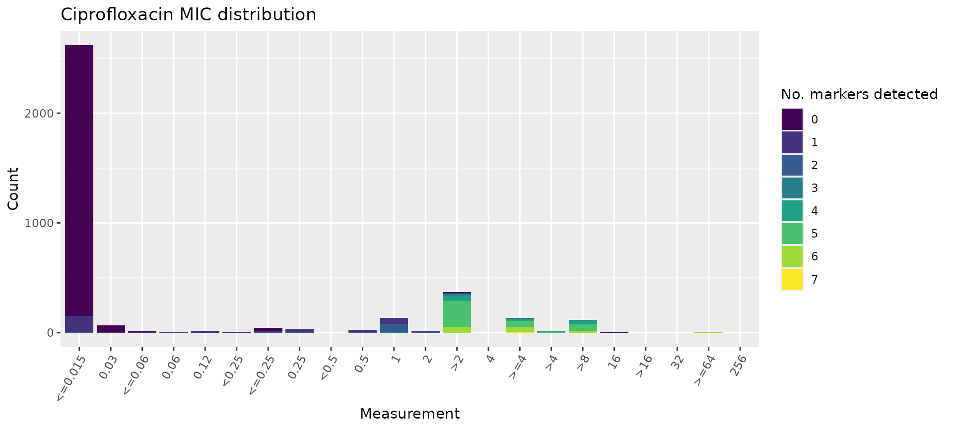
6. Model a binary drug phenotype using genetic marker presence/absence data
Logistic regression models can be informative to get an overview of the association between a drug resistance phenotype, and each marker thought to be associated with the relevant drug class.
The amr_logistic() function uses the
get_binary_matrix function to generate binary-coded
genotype and phenotype data for a specified drug and class; and fits two
logistic regression models of the form
R ~ marker1 + marker2 + marker3 + ... and
NWT ~ marker1 + marker2 + marker3 + ....
Note that the ‘NWT’ variable in the latter model can be taken either
from a precomputed ECOFF-based call of WT=wildtype/NWT=nonwildtype
(encoded in the input column ecoff_col), or computed from
the S/I/R phenotype as NWT=R/I and WT=S.
The amr_logistic() function can fit the model using
either the standard logistic regression approach implemented in the
glm() function, or Firth’s bias-reduced
penalized-likelihood logistic regression implemented in the
logistf package. The default is to use Firth’s regression,
as standard logistic regression can fail if there are too observations
in some subgroups, which happens quite often with this kind of data. To
use glm() instead, set glm=TRUE.
The function also filters out markers with too few observations in
the combined genotype/phenotype dataset. The default minimum is 10 but
this can be changed using the maf parameter (maf stands for
‘minor allele frequency’). If you are having trouble fitting models, it
may be because too many markers and combinations have very few
observations, and you might try increasing the maf value to
ensure that rare markers are excluded prior to model fitting.
Using this modelling approach, a negative association with a single marker and phenotype call of R and NWT is a strong indication that marker does not contribute to resistance. Note however that a positive association between a marker and R or NWT does not necessarily imply the marker is independently contributing to the resistance phenotype, as there may be non-independence between markers that is not adequately adjusted for by the model.
The function returns 4 objects:
modelR, modelNWT: data frames summarising each model, with beta coefficient, lower and upper values of 95% confidence intervals, and p-value for each marker (generated from the raw model output usinglogistf_details()orglm_details()as relevant)plot: a ggplot2 object generated from themodelRandmodelNWTobjects using thecompare_estimates()functionbin_mat: the binary matrix used as input to the regression models
# Manually run Firth's logistic regression model using the binary matrix produced above
dataR <- cip_bin[, setdiff(names(cip_bin), c("id", "pheno", "ecoff", "mic", "NWT"))]
dataR <- dataR[, colSums(dataR, na.rm = TRUE) > 5]
modelR <- logistf::logistf(R ~ ., data = dataR, pl = FALSE)
#> Warning in logistf::logistf(R ~ ., data = dataR, pl = FALSE): logistf.fit:
#> Maximum number of iterations for full model exceeded. Try to increase the
#> number of iterations or alter step size by passing 'logistf.control(maxit=...,
#> maxstep=...)' to parameter control

summary(modelR)
#> logistf::logistf(formula = R ~ ., data = dataR, pl = FALSE)
#>
#> Model fitted by Penalized ML
#> Coefficients:
#>                        coef  se(coef) lower 0.95 upper 0.95       Chisq
#> (Intercept)      -5.3126336 0.2631271 -5.8283532 -4.7969141         Inf
#> gyrA_S83L         5.0964769 0.3396242  4.4308257  5.7621280         Inf
#> gyrA_D87Y         0.6106668 1.9594688 -3.2298214  4.4511550  0.09712520
#> gyrA_D87N         1.0360455 1.2910108 -1.4942892  3.5663801  0.64401779
#> parC_S80I         3.5373730 1.2607416  1.0663649  6.0083812  7.87244336
#> parE_S458A       -0.6704877 1.4211494 -3.4558894  2.1149139  0.22258823
#> parC_S80R         0.9483222 0.9365007 -0.8871855  2.7838299  1.02540544
#> parE_L416F        1.0898410 1.4770169 -1.8050589  3.9847409  0.54444672
#> parC_S57T         1.4138484 1.4556144 -1.4391034  4.2668003  0.94343723
#> soxS_A12S         1.5835771 1.4858311 -1.3285984  4.4957527  1.13589853
#> parC_A56T         2.6649799 1.5169240 -0.3081365  5.6380963  3.08645711
#> qnrB19            5.2724510 0.4539251  4.3827740  6.1621279         Inf
#> `aac(6')-Ib-cr5`  4.2781111 1.3428296  1.6462134  6.9100089 10.14991218
#> parC_E84V        -0.5431447 1.7851855 -4.0420441  2.9557547  0.09256874
#> parE_I529L        2.0650647 0.4422569  1.1982571  2.9318724 21.80309146
#> parE_S458T       -2.7638947 1.9476308 -6.5811808  1.0533915  2.01386205
#> parE_E460D       -1.5247536 1.8858945 -5.2210388  2.1715317  0.65367903
#> parC_E84G         1.2138825 1.5879100 -1.8983640  4.3261290  0.58438832
#> qnrS1             5.5078662 0.4382199  4.6489710  6.3667613         Inf
#> marR_S3N          3.1497735 0.5128996  2.1445088  4.1550382 37.71325169
#> parE_I355T        1.9452320 0.8701522  0.2397651  3.6506990  4.99749513
#> soxR_G121D       -2.5711031 1.6085609 -5.7238245  0.5816183  2.55484162
#> qnrB4             6.9220299 1.5713224  3.8422946 10.0017653 19.40601369
#> parE_D475E       -0.7090156 1.4119171 -3.4763223  2.0582910  0.25216990
#>                             p method
#> (Intercept)      0.000000e+00      1
#> gyrA_S83L        0.000000e+00      1
#> gyrA_D87Y        7.553072e-01      1
#> gyrA_D87N        4.222596e-01      1
#> parC_S80I        5.019379e-03      1
#> parE_S458A       6.370749e-01      1
#> parC_S80R        3.112402e-01      1
#> parE_L416F       4.605957e-01      1
#> parC_S57T        3.313954e-01      1
#> soxS_A12S        2.865207e-01      1
#> parC_A56T        7.894653e-02      1
#> qnrB19           0.000000e+00      1
#> `aac(6')-Ib-cr5` 1.443081e-03      1
#> parC_E84V        7.609366e-01      1
#> parE_I529L       3.021130e-06      1
#> parE_S458T       1.558681e-01      1
#> parE_E460D       4.188004e-01      1
#> parC_E84G        4.445974e-01      1
#> qnrS1            0.000000e+00      1
#> marR_S3N         8.194598e-10      1
#> parE_I355T       2.538403e-02      1
#> soxR_G121D       1.099568e-01      1
#> qnrB4            1.056738e-05      1
#> parE_D475E       6.155513e-01      1
#>
#> Method: 1-Wald, 2-Profile penalized log-likelihood, 3-None
#>
#> Likelihood ratio test=3335.169 on 23 df, p=0, n=3630
#> Wald test = 515.415 on 23 df, p = 0

# Extract model summary details using `logistf_details()`
modelR_summary <- logistf_details(modelR)

modelR_summary
#> # A tibble: 24 × 5
#>    marker         est ci.lower ci.upper    pval
#>  * <chr>        <dbl>    <dbl>    <dbl>   <dbl>
#>  1 (Intercept) -5.31    -5.83     -4.80 0
#>  2 gyrA_S83L    5.10     4.43      5.76 0
#>  3 gyrA_D87Y    0.611   -3.23      4.45 0.755
#>  4 gyrA_D87N    1.04    -1.49      3.57 0.422
#>  5 parC_S80I    3.54     1.07      6.01 0.00502
#>  6 parE_S458A  -0.670   -3.46      2.11 0.637
#>  7 parC_S80R    0.948   -0.887     2.78 0.311
#>  8 parE_L416F   1.09    -1.81      3.98 0.461
#>  9 parC_S57T    1.41    -1.44      4.27 0.331
#> 10 soxS_A12S    1.58    -1.33      4.50 0.287
#> # ℹ 14 more rows
#> Use ggplot2::autoplot() on this output to visualise

# Plot the point estimates and 95% confidence intervals of the model
plot_estimates(modelR_summary)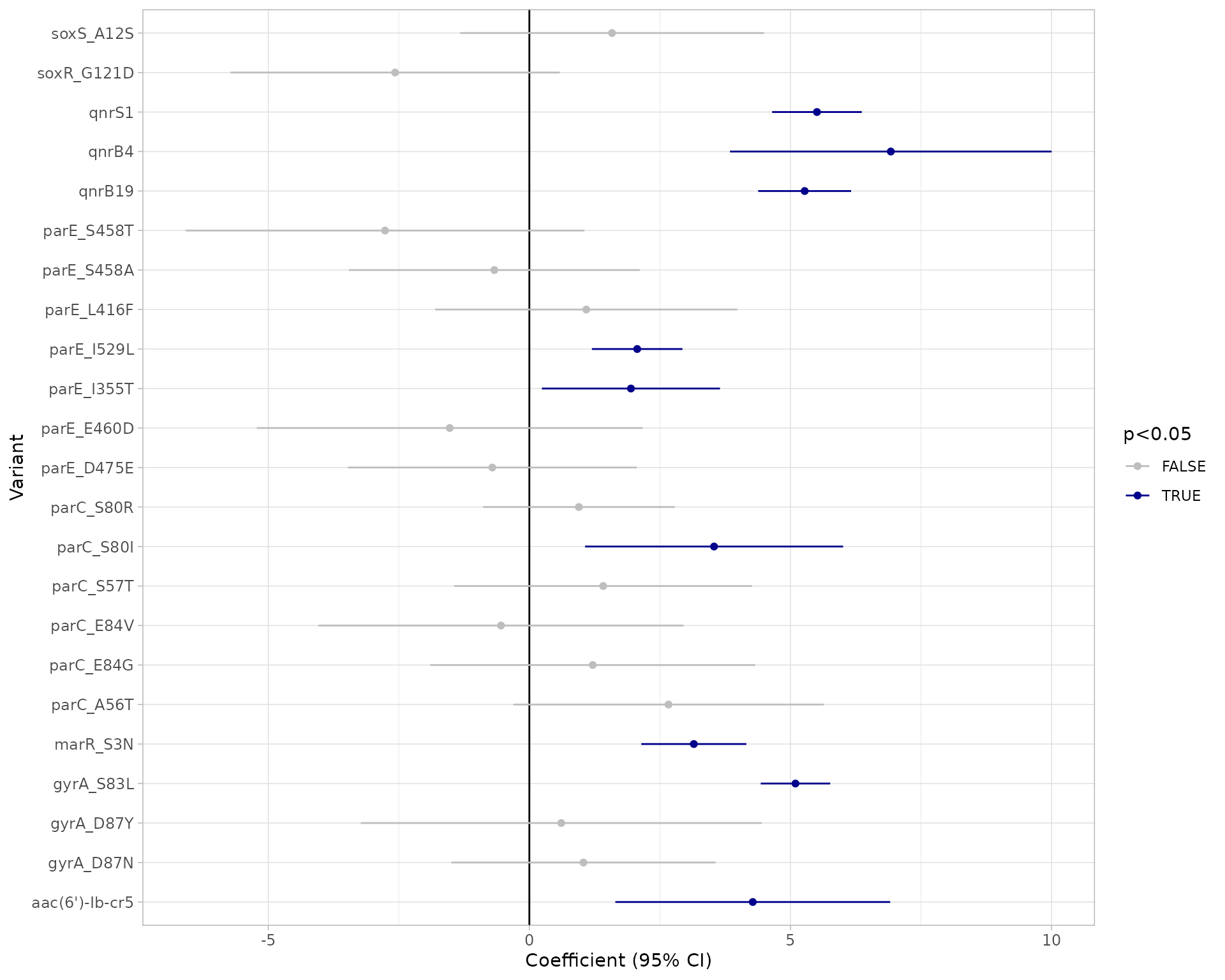
# Alternatively, use the amr_logistic() function to model R and NWT and plot the results together
models <- amr_logistic(
  geno_table = ecoli_geno,
  pheno_table = ecoli_ast,
  sir_col = "pheno_clsi",
  antibiotic = "Ciprofloxacin",
  drug_class_list = c("Quinolones"),
  maf = 10
)
#> Generating geno-pheno binary matrix
#>  Defining NWT in binary matrix using ecoff column provided: ecoff
#> ...Fitting logistic regression model to R using logistf
#>    Filtered data contains 3630 samples (793 => 1, 2837 => 0) and 19 variables.
#> Warning in logistf::logistf(R ~ ., data = to_fit, pl = FALSE): logistf.fit:
#> Maximum number of iterations for full model exceeded. Try to increase the
#> number of iterations or alter step size by passing 'logistf.control(maxit=...,
#> maxstep=...)' to parameter control
#> ...Fitting logistic regression model to NWT using logistf
#>    Filtered data contains 3630 samples (929 => 1, 2701 => 0) and 19 variables.
#> Warning in logistf::logistf(NWT ~ ., data = to_fit, pl = FALSE): logistf.fit:
#> Maximum number of iterations for full model exceeded. Try to increase the
#> number of iterations or alter step size by passing 'logistf.control(maxit=...,
#> maxstep=...)' to parameter control
#> Generating plots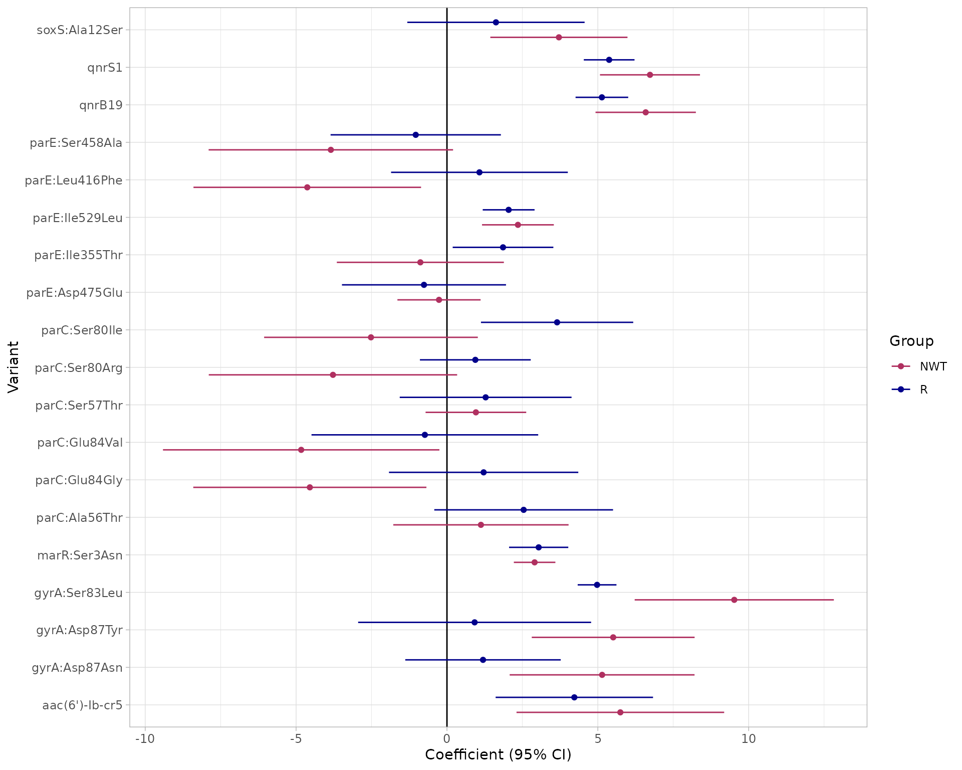
# Output tables
models$modelR
#> # A tibble: 20 × 5
#>    marker            est ci.lower ci.upper          pval
#>    <chr>           <dbl>    <dbl>    <dbl>         <dbl>
#>  1 (Intercept)    -5.18    -5.66     -4.70 0
#>  2 gyrA:Ser83Leu   4.98     4.33      5.62 0
#>  3 gyrA:Asp87Tyr   0.917   -2.94      4.78 0.642
#>  4 gyrA:Asp87Asn   1.19    -1.38      3.77 0.363
#>  5 parC:Ser80Ile   3.65     1.13      6.17 0.00457
#>  6 parE:Ser458Ala -1.03    -3.86      1.79 0.472
#>  7 parC:Ser80Arg   0.940   -0.896     2.78 0.316
#>  8 parE:Leu416Phe  1.08    -1.85      4.01 0.471
#>  9 parC:Ser57Thr   1.28    -1.57      4.13 0.377
#> 10 soxS:Ala12Ser   1.62    -1.31      4.56 0.279
#> 11 parC:Ala56Thr   2.54    -0.420     5.50 0.0926
#> 12 qnrB19          5.13     4.26      6.01 0
#> 13 aac(6')-Ib-cr5  4.22     1.61      6.83 0.00151
#> 14 parC:Glu84Val  -0.733   -4.49      3.02 0.702
#> 15 parE:Ile529Leu  2.04     1.19      2.90 0.00000311
#> 16 parC:Glu84Gly   1.22    -1.92      4.35 0.448
#> 17 qnrS1           5.38     4.54      6.22 0
#> 18 marR:Ser3Asn    3.04     2.06      4.02 0.00000000125
#> 19 parE:Ile355Thr  1.86     0.190     3.53 0.0290
#> 20 parE:Asp475Glu -0.761   -3.48      1.96 0.583
#> Use ggplot2::autoplot() on this output to visualise

models$modelNWT
#> # A tibble: 20 × 5
#>    marker            est ci.lower ci.upper     pval
#>    <chr>           <dbl>    <dbl>    <dbl>    <dbl>
#>  1 (Intercept)    -3.71    -3.97    -3.46  0
#>  2 gyrA:Ser83Leu   9.52     6.22    12.8   1.57e- 8
#>  3 gyrA:Asp87Tyr   5.51     2.81     8.21  6.29e- 5
#>  4 gyrA:Asp87Asn   5.14     2.08     8.21  1.00e- 3
#>  5 parC:Ser80Ile  -2.52    -6.06     1.02  1.63e- 1
#>  6 parE:Ser458Ala -3.85    -7.90     0.202 6.26e- 2
#>  7 parC:Ser80Arg  -3.78    -7.89     0.337 7.20e- 2
#>  8 parE:Leu416Phe -4.63    -8.40    -0.858 1.61e- 2
#>  9 parC:Ser57Thr   0.959   -0.709    2.63  2.60e- 1
#> 10 soxS:Ala12Ser   3.71     1.44     5.98  1.38e- 3
#> 11 parC:Ala56Thr   1.13    -1.78     4.03  4.48e- 1
#> 12 qnrB19          6.59     4.92     8.25  8.22e-15
#> 13 aac(6')-Ib-cr5  5.75     2.31     9.19  1.06e- 3
#> 14 parC:Glu84Val  -4.83    -9.41    -0.251 3.87e- 2
#> 15 parE:Ile529Leu  2.35     1.16     3.54  1.07e- 4
#> 16 parC:Glu84Gly  -4.54    -8.41    -0.681 2.11e- 2
#> 17 qnrS1           6.73     5.07     8.39  1.78e-15
#> 18 marR:Ser3Asn    2.91     2.22     3.59  1.11e-16
#> 19 parE:Ile355Thr -0.882   -3.65     1.89  5.32e- 1
#> 20 parE:Asp475Glu -0.263   -1.64     1.12  7.08e- 1
#> Use ggplot2::autoplot() on this output to visualise

# Note the matrix output is the same as cip_bin, but without the MIC data as this is not required
#    for logistic regression.
models$bin_mat
#> NULL
7. Assess solo positive predictive value of genetic markers
The strongest evidence of the effect of an individual genetic marker on a drug phenotype is its positive predictive value (PPV) for resistance amongst strains that carry this marker ‘solo’ with no other markers known to be associated with resistance to the drug class. This is referred to as ‘solo PPV’.
The function solo_ppv_analysis() takes as input our
genotype and phenotype tables, and calculates solo PPV for resistance to
a specific drug (included in our phenotype table) formarkers associated
with the specified drug class (included in our genotype table). It uses
the get_binary_matrix() function to first calculate the
binary matrix, then filters out all samples that have more than one
marker.
It then calculates for each remaining marker, amongst the genomes in which that marker is found solo, the number of genomes, the number and proportion that are R or NWT, and the 95% confidence intervals for these proportions. The values are returned as a table, and also plotted so we can easily visualise the distribution of S/I/R calls and the solo PPV for R and NWT, for each solo marker.
The function returns 4 objects:
solo_stats: data frame containing the numbers, proportions and confidence intervals for PPV of R and NWT categoriesamr_binary: the (wide format) binary matrix for all strains with geno/pheno data for the specified drug/classsolo_binary: the (long format) binary matrix for only those strains in which a solo marker was found, i.e. the data used to calculate PPVcombined_plot: a plot showing the distribution of S/I/R calls and the solo PPV for R and NWT, for each solo marker
# Run a solo PPV analysis
soloPPV_cipro <- solo_ppv_analysis(
  ecoli_geno,
  ecoli_ast,
  sir_col = "pheno_clsi",
  antibiotic = "Ciprofloxacin",
  drug_class_list = "Quinolones"
)
#> Generating geno-pheno binary matrix
#>  Defining NWT in binary matrix using ecoff column provided: ecoff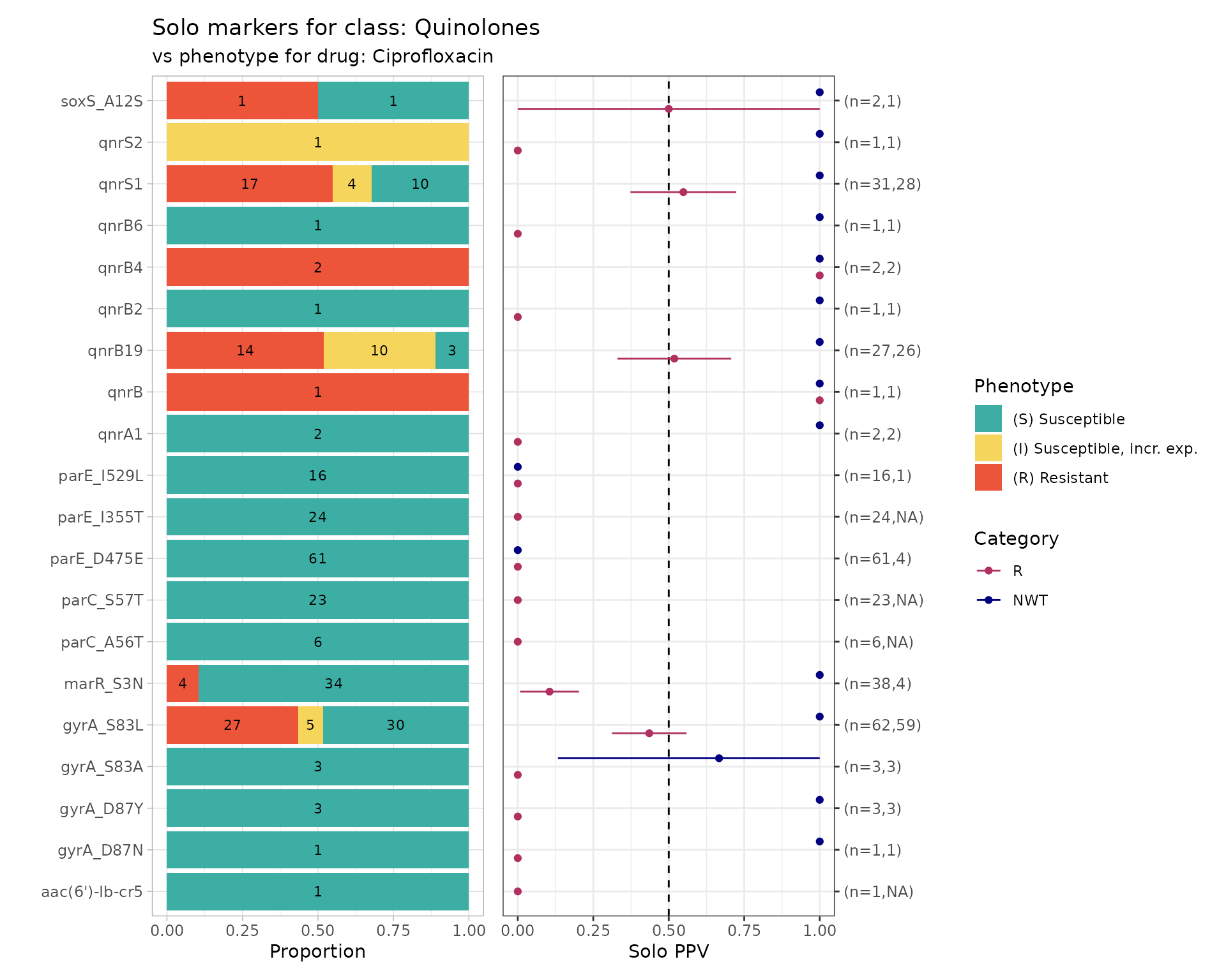
# Output table
soloPPV_cipro$solo_stats
#> # A tibble: 40 × 8
#>    marker         category     x     n   ppv     se ci.lower ci.upper
#>    <chr>          <chr>    <dbl> <int> <dbl>  <dbl>    <dbl>    <dbl>
#>  1 aac(6')-Ib-cr5 R            0     1 0     0       0          0
#>  2 gyrA_D87N      R            0     1 0     0       0          0
#>  3 gyrA_D87Y      R            0     3 0     0       0          0
#>  4 gyrA_S83A      R            0     3 0     0       0          0
#>  5 gyrA_S83L      R           27    62 0.435 0.0630  0.312      0.559
#>  6 marR_S3N       R            4    38 0.105 0.0498  0.00769    0.203
#>  7 parC_A56T      R            0     6 0     0       0          0
#>  8 parC_S57T      R            0    23 0     0       0          0
#>  9 parE_D475E     R            0    61 0     0       0          0
#> 10 parE_I355T     R            0    24 0     0       0          0
#> # ℹ 30 more rows

# Interim matrices with data used to compute stats and plots
soloPPV_cipro$solo_binary
#> # A tibble: 306 × 9
#>    id           pheno ecoff   mic  disk     R   NWT marker    value
#>    <chr>        <sir> <sir> <mic> <dsk> <dbl> <dbl> <chr>     <dbl>
#>  1 SAMN03177618   S     R    0.25    NA     0     1 gyrA_S83L     1
#>  2 SAMN03177619   S     R    0.12    NA     0     1 gyrA_D87Y     1
#>  3 SAMN03177623   S     R    0.25    NA     0     1 gyrA_S83L     1
#>  4 SAMN03177631   S     R    0.25    NA     0     1 gyrA_S83L     1
#>  5 SAMN03177635   S     R    0.25    NA     0     1 gyrA_S83L     1
#>  6 SAMN03177637   S     R    0.25    NA     0     1 gyrA_S83L     1
#>  7 SAMN03177638   S     R    0.25    NA     0     1 qnrB6         1
#>  8 SAMN03177639   S     R    0.12    NA     0     1 gyrA_S83L     1
#>  9 SAMN03177643   S     R    0.25    NA     0     1 gyrA_S83L     1
#> 10 SAMN03177646   S     R    0.25    NA     0     1 gyrA_S83L     1
#> # ℹ 296 more rows

soloPPV_cipro$amr_binary
#> # A tibble: 3,630 × 51
#>    id        pheno ecoff     mic  disk     R   NWT gyrA_S83L gyrA_D87Y gyrA_D87N
#>    <chr>     <sir> <sir>   <mic> <dsk> <dbl> <dbl>     <dbl>     <dbl>     <dbl>
#>  1 SAMN0317…   S     S   <=0.015    NA     0     0         0         0         0
#>  2 SAMN0317…   S     S   <=0.015    NA     0     0         0         0         0
#>  3 SAMN0317…   S     S   <=0.015    NA     0     0         0         0         0
#>  4 SAMN0317…   S     R     0.250    NA     0     1         1         0         0
#>  5 SAMN0317…   S     R     0.120    NA     0     1         0         1         0
#>  6 SAMN0317…   S     S   <=0.015    NA     0     0         0         0         0
#>  7 SAMN0317…   S     S   <=0.015    NA     0     0         0         0         0
#>  8 SAMN0317…   R     R    >4.000    NA     1     1         1         0         1
#>  9 SAMN0317…   S     R     0.250    NA     0     1         1         0         0
#> 10 SAMN0317…   R     R    >4.000    NA     1     1         1         0         1
#> # ℹ 3,620 more rows
#> # ℹ 41 more variables: parC_S80I <dbl>, parE_S458A <dbl>, parC_S80R <dbl>,
#> #   parE_L416F <dbl>, qnrB6 <dbl>, gyrA_D87G <dbl>, parC_S57T <dbl>,
#> #   parC_E84A <dbl>, soxS_A12S <dbl>, qnrB2 <dbl>, qnrS2 <dbl>,
#> #   parC_E84K <dbl>, parC_A56T <dbl>, qnrB19 <dbl>, `aac(6')-Ib-cr5` <dbl>,
#> #   parC_E84V <dbl>, parE_I529L <dbl>, parE_S458T <dbl>, parE_E460D <dbl>,
#> #   parC_E84G <dbl>, qnrS1 <dbl>, marR_S3N <dbl>, `aac(6')-Ib-cr` <dbl>, …
8. Compare markers with assay data
So far we have considered only the impact of individual markers, and their association with categorical S/I/R or WT/NWT calls.
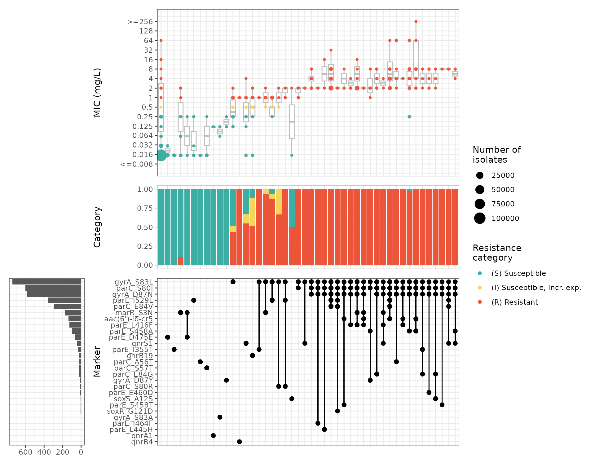
The function amr_upset() takes as binary matrix table
cip_bin summarising ciprofloxacin resistance vs quinolone
markers, generated using get_binary_matrix(), and explores
the distribution of MIC or disk diffusion assay values for all observed
combinations of markers (solo or multiple markers). It visualises the
data in the form of an upset plot, showing the distribution of assay
values and S/I/R calls for each observed marker combination, and returns
a summary of these distributions (including sample size, median and
interquartile range, number and proportion classified as R).
The function returns 2 objects:
summary: data frame containing summarising the data associated with each combination of markersplot: an upset plot showing the distribution of assay values, and breakdown of S/I/R calls, for each observed marker combination
# Compare ciprofloxacin MIC data with quinolone marker combinations,
#    using the binary matrix we constructed earlier via get_binary_matrix()
cipro_mic_upset <- amr_upset(
  cip_bin,
  min_set_size = 2,
  assay = "mic",
  order = "value"
)
# Output table
cipro_mic_upset$summary
#> # A tibble: 103 × 19
#>    marker_list        marker_count     n combination_id   R.n   R.ppv R.ci_lower
#>    <chr>                     <dbl> <int> <fct>          <dbl>   <dbl>      <dbl>
#>  1 ""                            0  2590 0_0_0_0_0_0_0…    10 0.00386    0.00147
#>  2 "qnrB"                        1     1 0_0_0_0_0_0_0…     1 1          1
#>  3 "parE_E460K, gyrA…            2     1 0_0_0_0_0_0_0…     1 1          1
#>  4 "parE_D475E"                  1    61 0_0_0_0_0_0_0…     0 0          0
#>  5 "qnrA1"                       1     2 0_0_0_0_0_0_0…     0 0          0
#>  6 "gyrA_S83A"                   1     3 0_0_0_0_0_0_0…     0 0          0
#>  7 "qnrB4"                       1     2 0_0_0_0_0_0_0…     2 1          1
#>  8 "parE_I355T"                  1    24 0_0_0_0_0_0_0…     0 0          0
#>  9 "marR_S3N"                    1    38 0_0_0_0_0_0_0…     4 0.105      0.00769
#> 10 "marR_S3N, parE_D…            2     4 0_0_0_0_0_0_0…     0 0          0
#> # ℹ 93 more rows
#> # ℹ 12 more variables: R.ci_upper <dbl>, NWT.n <dbl>, NWT.ppv <dbl>,
#> #   NWT.ci_lower <dbl>, NWT.ci_upper <dbl>, median_excludeRangeValues <dbl>,
#> #   q25_excludeRangeValues <dbl>, q75_excludeRangeValues <dbl>,
#> #   n_excludeRangeValues <int>, median_ignoreRanges <dbl>,
#> #   q25_ignoreRanges <dbl>, q75_ignoreRanges <dbl>